Chapter 4 Analysis of Algorithms

In the previous chapters we discussed how the hardware architectures we use (Chapter 2), the nature of the data we analyse and how we represent data with data structures (Chapter 3) contribute to the performance of a machine learning pipeline. The last major piece of this puzzle is the algorithmic complexity of the algorithms that power the machine learning models.

Algorithmic complexity is defined, in the abstract, as the amount of resources required by an algorithm to complete. After using pseudocode to write a high-level description of the machine learning algorithm we would like to implement (Section 4.1), we can determine the complexity of its components and how they contribute to the complexity of the algorithm as a whole. We represent and reason about complexity in mathematical terms with big-\(O\) notation (Section 4.2). Quantifying it (Section 4.3) presents several issues that are specific to machine learning (Section 4.4), which we will illustrate with three examples (Section 4.5).

4.1 Writing Pseudocode

The first step in reasoning about an algorithm is to write it down using pseudocode, combining the understandability of natural language and the precision of code to facilitate our analysis and the subsequent implementation in software. Natural language is easier to read, but it is also ambiguous. Code, on the other hand, is too specific: it forces us to think about implementation details and programming-language conventions thus making it harder to focus on the overall picture.

Pseudocode is meant to offset the weaknesses of natural language and code while preserving their strong points. Ideally, it provides a high-level description of an algorithm that facilitates its analysis and implementation by making the intent of each step clear while suppressing those details that are irrelevant for understanding the algorithm. There is no universal standard on how to write pseudocode, although some general guidelines exist (see, for instance, Chapter 9 in “Code Complete” (McConnell 2004)). The three key guidelines that are commonly accepted are:

• Each step of the algorithm should be a separate, self-contained item in an enumeration.
• Pseudocode should combine the styles of good code and of good natural language to some extent. For instance, it may fall short of full sentences. It should avoid idioms and conventions specific to any particular programming language, using a lax syntax for code statements. For the same reason, variable names should come from the domain of the problem the algorithm is trying to solve rather than from how they will be implemented (for instance, in terms of data structures). We will return to this point in Section 6.2.
• Pseudocode should ignore unnecessary details and use short-hand notation when possible, leaving the context to more in-depth forms of documentation. In other words, the level of detail should be that of a high-level view of the overall structure of the algorithm so that we can focus on its intent.

Admittedly, these recommendations are vague because the best way of conveying a high-level view of an algorithm to the reader depends on a combination of the pseudocode style and the reader’s background. As usual, knowing the audience is key in communicating effectively.

Writing good pseudocode for machine learning algorithms, or for machine learning pipelines spanning multiple algorithms, has two additional complications: the role played by the data and the need to integrate some amount of mathematical notation.

Firstly, if we are to treat data as code (Section 5.1), we may want to include more details about them in the pseudocode than we would in other settings. Such information may include, for example, the dimensions of the data and those characteristics of its features that are crucial for the algorithm to function. In a sense, this is similar to including some type information about key objects, and it is useful in clarifying what the inputs and the outputs of the algorithm are as well as in giving more context to key steps.

Secondly, mathematical notation may be the best tool to describe key steps in a clear and readable way, so we may want to integrate it with natural language and code to the best effect. In order to do that, we should define all the variables and the functions used in the notation while leaving additional details to a separate document. For practical purposes, mentioning the meaning of each symbol when introducing new mathematical notation (for instance, “the prior Beta distribution \(\pi(\alpha, \beta) \sim \mathit{Be}(\alpha, \beta)\)” as opposed to just “\(\pi(\alpha, \beta) \sim \mathit{Be}(\alpha, \beta)\)”) is often enough to give context (what are properties of \(\pi\), how it will be used, etc.). Complex formulas, derivations and formal proofs would reduce the readability of pseudocode by making it overlong and forcing the reader to concentrate on understanding them instead of looking at the overall logic of the algorithm.

Describing all algorithms used in a machine learning pipeline using pseudocode has some further advantages we will touch on in later chapters:

• it makes code review easier (see Section 6.6);
• it facilitates iterative refinement because pseudocode is easier to modify than code (see Section 5.3.1);
• it provides design documentation in a form that is easy to maintain (see Section 8.3).

4.2 Computational Complexity and Big-\(O\) Notation

Computational complexity is a branch of computer science that focuses on classifying computational problems according to their inherent difficulty across three different dimensions:

• as a function of input size (say, the sample size or the number of variables);
• as a function of how much resources will be used, in particular time (say, CPU time spent) and space (memory or storage use);
• on average (how long it will typically take), in the best case or in the worst case (how long it can possibly take).

In other words, we would like to infer how much resources an algorithm will use just from its specification: this is called algorithm analysis. Typically, the specification takes the form of pseudocode. As for the resources, we must first choose our unit of measurement. In the case of space complexity, the choice is usually obvious: either an absolute memory unit (such as MB, GB) or a relative one (such as the number of double-precision floating point values) for various types of memory (RAM, GPU memory, storage). In the case of time complexity, we must choose a set of fundamental operations that we consider to have a theoretical complexity of \(1\). Such operations can range from simple (arithmetic operations) to complex (models trained) depending on the level of abstraction we would like to work at. On the one hand, the lower the level of abstraction, the more we need to know about the specific implementation details of the algorithm. This is only feasible up to a point because pseudocode will omit most such details. It is also undesirable to some extent because it makes the analysis less general: a different implementation of the same algorithm may end up in a different class of complexity while exhibiting about the same behaviour in practice. On the other hand, the higher the level of abstraction, the higher the chance of obtaining an estimate of complexity that is only loosely connected to reality. The more complex the operations, the more unlikely it will be that they have the same complexity and that their complexity can be taken to be constant.

The estimates of computational complexity produced by algorithm analysis are written using big-\(O\) and related notations, which define the class of complexity in the limit of the input sizes (Knuth 1976, 1997). (All algorithms are fast with small inputs.) More in detail:

• We describe the worst-case scenario using big-\(O\) notation. Formally, an algorithm with input of size \(N \to \infty\) has a complexity \(f(N) = O(g(N))\) if there exists a \(c_0 > 0\) such that \(f(N) \leqslant c_0 g(N)\). It represents an upper bound in complexity.
• We describe the best-case scenario using big-\(\Omega\) notation: \(f(N) = \Omega(g(N))\), \(f(N) \geqslant c_1 g(N)\) with \(c_1 > 0\). It represents a lower bound in complexity.
• We describe the average case using big-\(\Theta\) notation: \(f(N) = \Theta(g(N))\), \(c_2 g(N) \leqslant f(N) \leqslant c_3 g(N)\) with \(c_2, c_3 > 0\). It represents the average complexity.

In practice, we often just write things like “it is \(O(g(N))\) on average and \(O(h(N))\) in the worst case” and use big-\(O\) for all three cases. If we are considering inputs that are best described with a combination of different sizes (say, \(\{M, N, P\}\)), big-\(O\) will be a multivariate function like \(O(g(M, N, P))\).

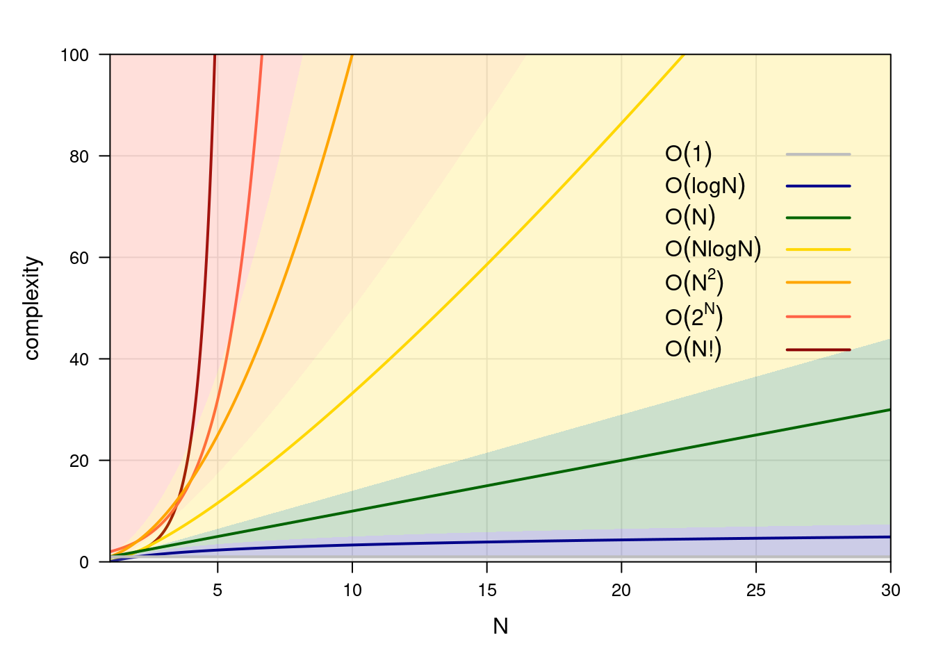
Figure 4.1: A graphical comparison of computational complexity classes.

Different classes of complexity in common use are shown in Figure 4.1. Algorithms that belong to \(O(1)\), \(O(\log N)\), \(O(N)\) and \(O(N \log N)\) are considered efficient, while those that belong to \(O(N^2)\) or higher classes of complexity are more demanding. In a sense, this classification reflects the economics of running compute systems: it may be feasible to double our hardware requirements every time \(N\) doubles, but increasing it by a power of 2 or more is rarely possible!

How can we use big-\(O\) notation? If we are comparing algorithms in different classes of complexity, we can concentrate only on the leading term: \(O(3 \cdot 2^N + 3.42 N^2) \gg O(2 N^3 + 3 N^2)\) is functionally equivalent to \(O(2^N) \gg O(N^3)\) because the difference in the order of magnitude makes lower-order terms and even the coefficient of the leading term irrelevant. If we are comparing algorithms in the same class of complexity, we only report the leading term and its coefficient: \(O(1.2 N^2 + 3N) \gg O(0.9 N^2 + 2 \log N)\) becomes \(O(1.2 N^2) \gg O(0.9 N^2)\). In the former case, we can say algorithms scale in fundamentally different ways as their inputs grow in size. In the latter, we can say that algorithms scale similarly but still rank them.

In most practical settings, however, interpreting big-\(O\) notation requires a more nuanced approach because of its intrinsic limitations.

• Big-\(O\) notation does not include constant terms, so it may not necessarily map well to real-world performance. Algorithms with complex initialisation phases that do not scale with input sizes may be slower than algorithms with higher complexity for even moderate input sizes. This may be the case of algorithms that cache partial results or sufficient statistics when the caching is more expensive than recomputing those quantities from scratch as needed.
• Similarly, the coefficients in big-\(O\) notation are usually not realistic: for instance, a time complexity \(O(2N)\) does not guarantee that doubling \(N\) will double running time. How the algorithm is implemented, on what hardware, etc. may not affect the class of complexity but they always have a strong effect on the associated coefficients. As a result, we should estimate those coefficients from empirical run-times to obtain realistic performance curves, and use the latter to compare algorithms within the same class of complexity.
• There is a compromise between space and time complexity: we trade off one for the other. Arguably, space complexity is more important than time complexity. In principle, we can wait a bit longer to get the results, but if our program runs out of memory, it will crash and we will get no results at all.

4.3 Big-\(O\) Notation and Benchmarking

Producing empirical performance curves for all relevant dimensions of computational complexity differs from other forms of benchmarking in a few ways. If we know the theoretical class of complexity an algorithm belongs to, a simple linear model will suffice for estimating the coefficients of the terms in its big-\(O\) notation: we will show some examples in Section 4.5. However, we should take some care in how performance is measured and in how we interpret the empirical curves.

Firstly, we should plan the collection of the performance measurements following the best practices in the design of physical (Montgomery 20AD) and computer simulation (Santner, Williams, and Notz 2018) experiments. If we are measuring complexity along a single dimension, we should collect multiple performance measurements for each input size. The average performance at each input size will provide a more stable estimate than a single measurement, and we can use the distribution of the performance measurements to establish confidence bands around the average. Bands based on empirical quantiles (say, the interval between the [5%, 95%] quantiles) are often preferable to bands based on the quantiles of the normal distribution (say, average performance \(\pm\) the standard deviation times the 95% quantile of the standard normal) because the latter is symmetric around the average and fails to account for the fact that performance is skewed. Performance is naturally bounded below by zero (instant execution!) and the average performance may be close enough to zero that the bottom of the confidence band is negative!

If we are measuring complexity along multiple dimensions, it is best to use a single experimental design that involves all of them in order to separate the main effect of each dimension from their interactions. Big-\(O\) notation may not include terms that contain more than one dimension, and in that case it is interesting to check whether that is true in practice as well. Or big-\(O\) notation may include such terms, and then the only consistent way of estimating their coefficients is to vary all the involved input sizes simultaneously.

If we are comparing two algorithms in the same complexity class, we should do that on performance differences generated on the same sets of inputs to increase the precision of our comparison. If we use different inputs, the performance measures we collect for each input size are independent across algorithms: if those algorithms are \(O(f(N))\) and \(O(g(N))\) respectively, \[\begin{equation*} \operatorname{VAR}(f(N) - g(N)) = \operatorname{VAR}(f(N)) + \operatorname{VAR}(g(N)). \end{equation*}\] However, if we use the same inputs for both algorithms \[\begin{multline*} \operatorname{VAR}(f(N) - g(N)) = \operatorname{VAR}(f(N)) + \operatorname{VAR}(g(N)) - \\ 2\operatorname{COV}(f(N), g(N)) \end{multline*}\] because the performance measures are no longer independent. Since \(\operatorname{COV}(f(N), g(N)) > 0\), the empirical differences in performance will have smaller variability and thus greater precision.

Secondly, we should carefully choose the compute system we use. The system should “stand still” while we are taking performance measurements: if other tasks are running at the same time, they may try to access shared resources that are also involved in our performance measures. This has two negative effects: it makes performance measures noisier and it inflates the estimated coefficients by making the average performance worse.

Thirdly, we should be careful in using performance curves to predict performance outside the range of the input sizes (or the combinations of input sizes) we actually measured. In any compute system with finite resources, resource contention will increase as the system reaches saturation. Hence we should use a compute system with enough resources to handle all the input sizes we consider without going anywhere near capacity. We are interested in measuring the performance of the algorithm, not of the compute system, so we should put stress on the former and not on the latter.

Finally, note that most experimental design approaches assume that performance measures are independent. Hence we should strive to make our empirical measures as independent as possible by resetting the state of the compute system before each run: for instance, we should remove all temporary objects.

4.4 Algorithm Analysis for Machine Learning

Algorithm analysis presents some additional complications in the context of machine learning software.

The first set of complications is related to defining the size of the input. Machine learning algorithms typically have a large number of different inputs, and the size of each input has several dimensions (such as the sample size and the number of variables). Hence algorithms will belong to different classes of complexity for different dimensions, and it will be unlikely that any will dominate the others in all dimensions. Sometimes we can reduce the number of dimensions we are considering by assuming some are bounded because of the intrinsic nature of the inputs or by expressing one dimension as a function of another (say, the number of variables is \(p \approx \sqrt{n}\) where \(n\) is the sample size).

Furthermore, computational complexity depends strongly on the assumptions we make on the distributions of the inputs and not just on their sizes. More assumptions usually allow us to access algorithms with better performance, and make it possible to use closed-form results: the more knowledge we put in the form of assumptions, the less we have to learn empirical measures. Assuming some form of sparsity or regularity, or actively enforcing it in the learning process, will reduce the complexity of machine learning models to the point they become tractable. In most settings, not making any such assumption will mean exponential or combinatorial worst-case complexity. It is another trade-off: assumptions versus complexity.

For stochastic algorithms, we can only meaningfully reason on the average case. Consider Markov chain Monte Carlo (MCMC) posterior inference in Bayesian models, or stochastic gradient descent (SGD) for deep neural networks. Each time we run them, they go through a different sequence of steps and they may produce a different posterior distribution or model. As a consequence, each run will take a different amount of time and it will use a different amount of memory. The construction of such algorithms gives convergence guarantees and convergence rates, so we have some expectations about average complexity, but there is always some degree of uncertainty.

4.5 Some Examples of Algorithm Analysis

We will now apply the concepts we just introduced by investigating the time complexity of estimating the coefficients of linear regression models (Section 4.5.1); the trade-off between time and space complexity in sparse matrices (Section 4.5.2); and the time and space complexity of an MCMC algorithm to generate random directed acyclic graphs from a uniform distribution (Section 4.5.3).

4.5.1 Estimating Linear Regression Models

Linear models are the foundation upon which most of statistics and machine learning are built: we often use them either as standalone models or as part of more complex ones. Generally speaking, a linear model takes a vector \(\mathbf{y}\) and a matrix \(\mathbf{X}\) of real numbers and tries to explain \(\mathbf{y}\) as a function of \(\mathbf{X}\) that is linear in the parameters \(\boldsymbol{\beta}\). We can famously (Weisberg 2014) estimate \(\boldsymbol{\beta}\) with the closed-form expression \[\begin{equation*} \underset{p \times 1}{\boldsymbol{\widehat{\beta}}_{\mathrm{EX}}} = (\underset{p \times n}{\mathbf{X}^\mathrm{T}\vphantom{\boldsymbol{\widehat{\beta}}_{\mathrm{EX}}}} \, \underset{n \times p}{\mathbf{X}\vphantom{\boldsymbol{\widehat{\beta}}_{\mathrm{EX}}}})^{-1} \underset{p \times n}{\mathbf{X}^\mathrm{T}\vphantom{\boldsymbol{\widehat{\beta}}_{\mathrm{EX}}}} \, \underset{n \times 1}{\mathbf{y}} \end{equation*}\] which is, at the same time, the ordinary least squares estimate (from the orthogonal projection of \(\mathbf{y}\) onto the space spanned by the \(\mathbf{X}\)) and the maximum likelihood estimate of \(\boldsymbol{\beta}\) (under the assumption residuals are independent and normally distributed with a common variance). Note how we have annotated the formula above with the dimensions of both \(\mathbf{X}\) and \(\mathbf{y}\). Those are our inputs: their dimensions depend on the sample size \(n\) and on the number of variables \(p\).⁹ The algorithmic complexity of estimating \(\boldsymbol{\beta}\) will be a function of both.

Another option to estimate \(\boldsymbol{\beta}\) is to use the QR decomposition of \(\mathbf{X}\) (Weisberg 2014, Appendix A.9). Starting from the \(\mathbf{X}\boldsymbol{\beta}= \mathbf{y}\) formulation of the linear regression model, we perform the following steps:

1. compute the QR decomposition of \(\mathbf{X}\) (\(\mathbf{Q}\) is \(n \times p\), \(\mathbf{R}\) is \(p \times p\));
2. rewrite the problem as \(\mathbf{R} \boldsymbol{\beta}= \mathbf{Q}^\mathrm{T}\mathbf{y}\);
3. compute \(\mathbf{Q}^\mathrm{T}\mathbf{y}\);
4. solve the resulting (triangular) linear system for \(\boldsymbol{\beta}\).

Let’s call this estimator \(\boldsymbol{\widehat{\beta}}_{\mathrm{QR}}\). If we discount numerical issues with pathological \(\mathbf{X}\)s, \(\boldsymbol{\widehat{\beta}}_{\mathrm{QR}}\) and \(\boldsymbol{\widehat{\beta}}_{\mathrm{EX}}\) give identical estimates of \(\boldsymbol{\beta}\): they are identical in terms of statistical properties, and neither makes any assumption of the distribution of \(\mathbf{X}\). However, we may still prefer one to the other because of their time complexity.

Firstly, what is the time complexity of computing \(\boldsymbol{\widehat{\beta}}_{\mathrm{EX}}\)? The steps we would perform if we were estimating it by hand are:

1. compute \(\mathbf{X}^\mathrm{T}\mathbf{X}\);
2. invert it and compute \((\mathbf{X}^\mathrm{T}\mathbf{X})^{-1}\);
3. compute \(\mathbf{X}^\mathrm{T}\mathbf{y}\);
4. multiply the results from steps 2 and 3.

Given the simplicity of \(\boldsymbol{\widehat{\beta}}_{\mathrm{EX}}\), this description will suffice as the pseudocode for our analysis. From easily available sources (say, Wikipedia), we can find the time complexity of the operation in each step:

• multiplying an \(r \times s\) matrix and an \(s \times t\) matrix takes \(O(rst)\) operations (Wikipedia 2021b);
• computing the inverse of an \(r \times r\) matrix is \(O(r^3)\) using a Cholesky decomposition (Wikipedia 2021a) or Gram-Schmidt (Wikipedia 2021c).

These time complexities use arithmetic operations as the elementary operations, which is natural because matrices are just sets of numbers that are combined and transformed using those operations. The actual contents of \(\mathbf{X}\) and \(\mathbf{y}\) are irrelevant: both matrices appear in the big-\(O\) notation just with their dimensions.

Therefore, step 1 is \(O(pnp) = O(np^2)\), step 2 is \(O(p^3)\), step 3 is \(O(np)\) and step 4 is \(O(p^2)\). The overall time complexity is \[\begin{equation} O(np^2 + p^3 + np + p^2) = O(p^3 + (n + 1)p^2 + np) \tag{4.1} \end{equation}\] and it can be interpreted as follows:

• Estimating \(\boldsymbol{\widehat{\beta}}_{\mathrm{EX}}\) is \(O(p^3)\) in the number of parameters \(p\): if \(p\) doubles, it takes eight times as long.
• Estimating \(\boldsymbol{\widehat{\beta}}_{\mathrm{EX}}\) is \(O(n)\) in the sample size \(n\): if \(n\) doubles, it takes twice as long.

Let’s look now at \(\boldsymbol{\widehat{\beta}}_{\mathrm{QR}}\). For time complexity we have that:

• solving an \(r \times s\) linear system with Gram-Schmidt is \(O(rs^2)\);¹⁰
• back-substitution to solve the triangular linear system in step 4 is \(O(s^2)\).

Therefore, step 1 is \(O(np^2)\), step 3 is \(O(np)\) and step 4 is \(O(p^2)\). (Step 2 is merely for notation.) The overall time complexity is then \[\begin{equation} O(np^2 + np + p^2) = O((n + 1)p^2 + np), \tag{4.2} \end{equation}\] making \(\boldsymbol{\widehat{\beta}}_{\mathrm{QR}}\) quadratic in the number of parameters and linear in the sample size. We can expect it to be faster than the closed-form estimator as \(p\) grows (\(O(p^2)\) instead of \(O(p^3)\)), but we cannot say which approach is faster as \(n\) grows because they are both \(O(n)\).

Therefore, which algorithm is best depends on the data we expect to work on:

• if \(n \to \infty\) but \(p\) is bounded, \(\boldsymbol{\widehat{\beta}}_{\mathrm{EX}}\) and \(\boldsymbol{\widehat{\beta}}_{\mathrm{QR}}\) perform similarly well;
• if \(p \to \infty\), \(\boldsymbol{\widehat{\beta}}_{\mathrm{QR}}\) will be faster.

How well do the time complexities in (4.1) and (4.2) map to real-world running times? We can answer this question by benchmarking \(\boldsymbol{\widehat{\beta}}_{\mathrm{EX}}\) and \(\boldsymbol{\widehat{\beta}}_{\mathrm{QR}}\) as we discussed in Section 4.3.

library(microbenchmark)
library(doBy)

# define the estimators.
betaEX = function(y, X) solve(crossprod(X)) %*% t(X) %*% y
betaQR = function(y, X) qr.solve(X, y)
# define the grid of input sizes to examine.
nn = c(1, 2, 5, 10, 20, 50, 100) * 1000
pp = c(10, 20, 50, 100, 200, 500)
# a data frame to store the running times.
time = data.frame(
  expand.grid(n = nn, p = pp, betahat = c("EX", "QR")),
  lq = NA, mean = NA, uq = NA
)
# quantiles defining a 90% confidence band.
lq = function(x) quantile(x, 0.05)
uq = function(x) quantile(x, 0.95)
# for all combinations of input sizes...
for (n in nn) {
  for (p in pp) {
    # ... measure the running time averaging over 100 runs...
    bench = microbenchmark(betaEX(y, X), betaQR(y, X),
              times = 100,
              control = list(warmup = 10),
              setup = {
                X = matrix(rnorm(n * p), nrow = n, ncol = p)
                y = X %*% rnorm(ncol(X))
              })
    # ... and save the results for later analyses.
    time[time$n == n & time$p == p, c("lq", "mean", "uq")] =
      summaryBy(time ~ expr, data = bench,
                FUN = c(lq, mean, uq))[, -1]
  }#FOR
}#FOR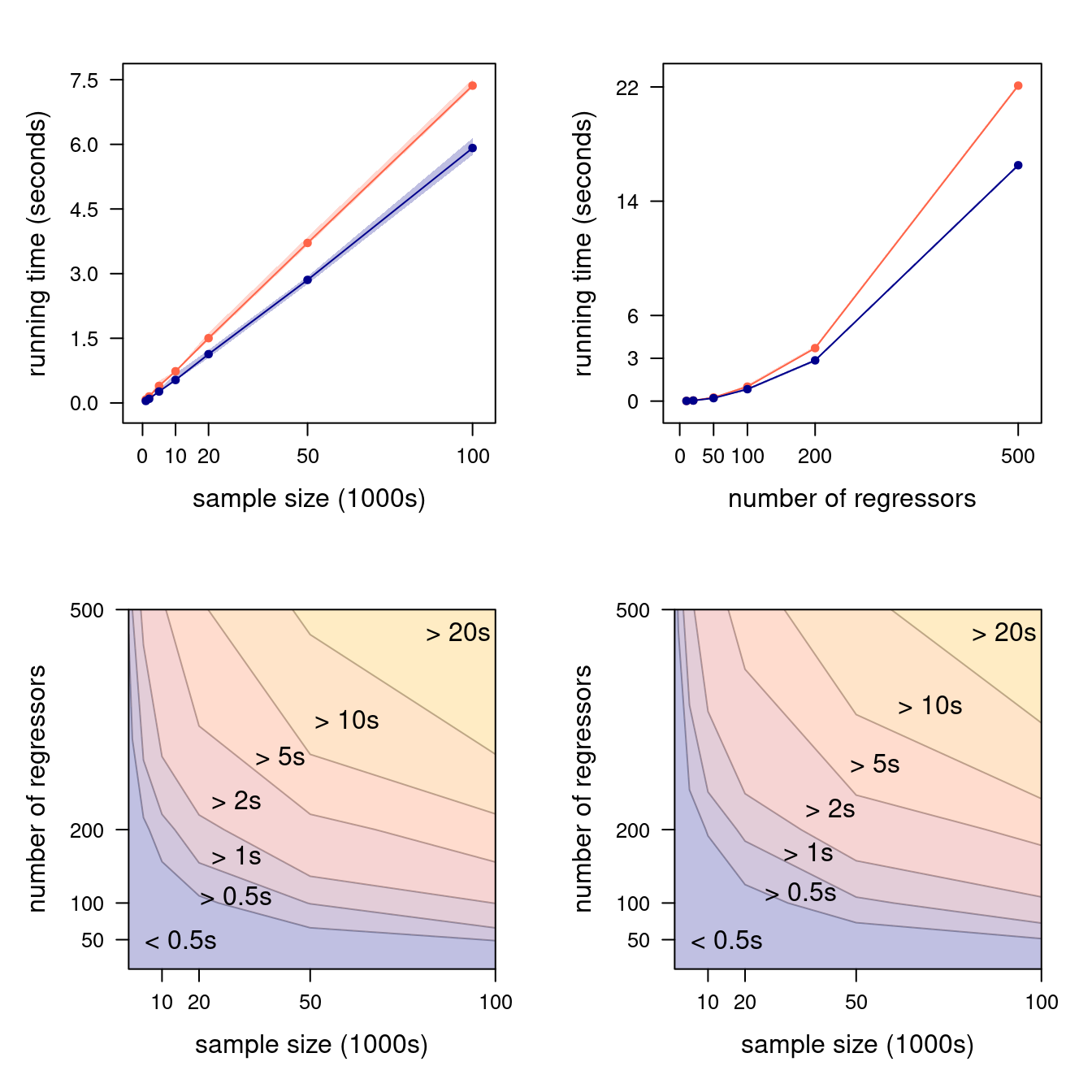

Figure 4.2: Marginal running times as a function of \(n\) (with \(p = 200\), top left) and of \(p\) (with \(n = 50000\), top right); the closed-form formula is shown in orange and the QR estimator in blue, each with 90% confidence bands. Joint running times in \((n, p)\) are shown in the bottom left and right panels for the closed-form formula and the QR estimator, respectively.

We plotted the results in Figure 4.2. The top panels confirm the conclusions we reached earlier: both \(\boldsymbol{\widehat{\beta}}_{\mathrm{EX}}\) and \(\boldsymbol{\widehat{\beta}}_{\mathrm{QR}}\) have a time complexity that is linear in \(n\), hence they scale similarly; but \(\boldsymbol{\widehat{\beta}}_{\mathrm{EX}}\) has a cubic time complexity in \(p\), which makes it much slower than \(\boldsymbol{\widehat{\beta}}_{\mathrm{QR}}\) as \(p\) increases. The level plots in the bottom panels show that \(n\) and \(p\) jointly influence running times, which we should expect since both (4.1) and (4.2) contain mixed terms in which both \(n\) and \(p\) appear.

Considering how little noise is in the running times we measured, we can reliably estimate the coefficients of the terms in (4.1) and (4.2) using a simple linear regression.

# rescale to make the coefficients easier to interpret.
time$mean = time$mean * 10^(-9)
time$n = time$n / 1000
bigO.EX = lm(mean ~ I(p^3) + I((n + 1) * p^2) + I(n * p),
             data = subset(time, betahat == "EX"))
coefficients(bigO.EX)

##      (Intercept)           I(p^3) I((n + 1) * p^2)
##    -0.0120329302    -0.0000000025     0.0000017156
##         I(n * p)
##     0.0000244271

bigO.QR = lm(mean ~ I((n + 1) * p^2) + I(n * p),
             data = subset(time, betahat == "QR"))
coefficients(bigO.QR)

##      (Intercept) I((n + 1) * p^2)         I(n * p)
##       -0.1103315        0.0000013        0.0000502

The models in bigO.EX and bigO.QR allow us to predict the running times for any combinations of \(n\) and \(p\). We can also use them to check how much the empirical complexity curves they encode overlap the corresponding empirical running times and check for outliers.

As a final note, there are several additional considerations we should weigh before choosing which algorithm to use: the matrix inverse in \(\boldsymbol{\widehat{\beta}}_{\mathrm{EX}}\) is known to be numerically unstable, which is why \(\boldsymbol{\widehat{\beta}}_{\mathrm{QR}}\) is preferred in scientific software. lm() in both R and Julia, fitlm() in MATLAB are implemented on top of QR but, interestingly, LinearRegression() in Scikit-learn (Scikit-learn Developers 2022) is not.

4.5.2 Sparse Matrices Representation

Matrices in which most cells are zero are called sparse matrices, as opposed to dense matrices in which most or all elements are non-zero. In the case of dense (\(m \times n\)) matrices, we need to store in memory the values of all the cells, which means that their complexity is \(O(mn)\). However, in the case of sparse matrices, we can just store the non-zero values and their coordinates, with the understanding that all other cells are equal to zero.

R provides several such representations in the Matrix package (Bates and Maechler 2021), and Python does the same in scipy (Virtanen et al. 2020): the default is the column-oriented, compressed format described in Section 3.2.3. Consider the matrix originally shown in Figure 3.4, in which 9 cells out of 15 are zeroes.

library(Matrix)
m = Matrix(c(0, 0, 2:0), 3, 5)
m

## 3 x 5 sparse Matrix of class "dgCMatrix"
##
## [1,] . 1 . . 2
## [2,] . . 2 . 1
## [3,] 2 . 1 . .

How are the elements of m stored in memory?

str(m)

## Formal class 'dgCMatrix' [package "Matrix"] with 6 slots
##   ..@ i       : int [1:6] 2 0 1 2 0 1
##   ..@ p       : int [1:6] 0 1 2 4 4 6
##   ..@ Dim     : int [1:2] 3 5
##   ..@ Dimnames:List of 2
##   .. ..$ : NULL
##   .. ..$ : NULL
##   ..@ x       : num [1:6] 2 1 2 1 2 1
##   ..@ factors : list()

Comparing the notation in Section 3.2.3 and the documentation of Matrix, we can see that:

• i contains the vector \(R\), row coordinates of the non-zero cells in the matrix;
• p contains the vector \(C\), the start and end indexes of the columns; and
• x contains the vector \(V\) of the values of the non-zero cells.

Note that both i and p are 0-based indexes to facilitate the use of the dgCMatrix class in the code inside the Matrix package, while R uses 1-based indexing.

The overall space complexity of such a sparse matrix is then \(O(3z)\), where \(z\) is the number of non-zero cells. R stores real numbers in double precision (64 bits each) and indexes as 32-bits integers, which means m needs 128 bits (16 bytes) of memory for each non-zero cell. So dense matrices use \(8mn\) bytes of memory while sparse matrices use \(16z\) bytes; if \(z \ll mn\) we can save most of the memory we would have allocated for a dense matrix.

The catch is that operations may have a higher time complexity for sparse matrices than for dense matrices. Even the most simple: looking up the value of a cell \((i, j)\) has time complexity \(O(1)\) in a dense matrix, but for a sparse matrix such as m we need to:

• Look up what are the first and the last values in x for the column \(j\) by reading the \(j\)th element of p.
• Position ourselves on the row number for that first value in i, and read every successive number until we find the row number \(j\) or we reach the end of the column.
• Read the value of the cell from x, which has the same position in x as the row number in i; or return zero if we reach the end of the column.

These three steps have an overall time complexity of \(O(1) + O(z/n) + O(1) = O(2 + z/n)\) assuming \(z/n\) non-zero elements per column on average. Hence reading a cell from a sparse matrix appears to be more expensive than reading the same cell from a dense matrix.

Assigning a non-zero value to a cell in a sparse matrix is more expensive as well. For each of i and x we need to:

• allocate a new array of length \(z + 1\);
• copy the \(z\) values from the old array;
• add the values corresponding to the new cell;
• replace the old array with the new one.

Therefore, time and space complexity both are \(O(z)\). Handling p is also \(O(z)\), and it is more complex since we will need to recompute half of the values on average.

This is troubling because we cannot predict the average time and space complexity just by looking at the input size: we can only do that by making assumptions on the distribution of the values in the cells. Furthermore, this distribution may change during the execution of our software as we assign new non-zero values to the sparse matrix. We can, however, compare the empirical running times of read and write operations on dense and sparse matrices to get a practical understanding of how they differ, as we did in the previous section with \(\boldsymbol{\widehat{\beta}}_{\mathrm{EX}}\) and \(\boldsymbol{\widehat{\beta}}_{\mathrm{QR}}\).

Consider a square matrix allocated as either a sparse or a dense matrix with \(n = 1000\) and the proportions of non-zero cells of \(z/n = \{ 0.01, 0.02, 0.05,\) \(0.10, 0.20, 0.50, 1\}\). We can measure the time it takes to read (with the read10() function) or write (with the write10() function) the values of 10 random cells for either type of matrix as \(z\) (zz in the code below) increases.

read10 = function(m) m[sample(length(m), 10)]
write10 = function(m) m[sample(length(m), 10)] = 1
[...]
for (z in zz) {
  bench = microbenchmark(
            read10(sparse), read10(dense),
            write10(sparse), write10(dense),
            times = 200,
            control = list(warmup = 10),
            setup = {
              sparse = Matrix(0, n, n)
              sparse[sample(length(sparse), round(z))] = 1
              dense = matrix(0, n, n)
            })
  [...]
}#FOR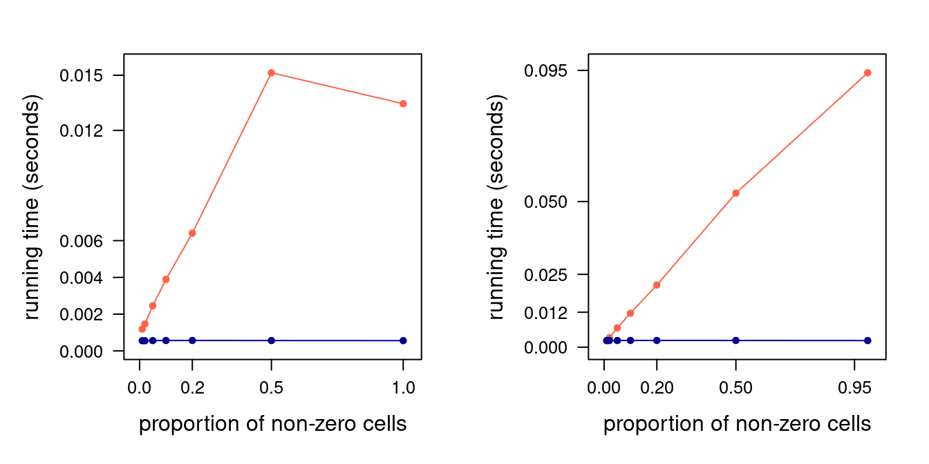

Figure 4.3: Read (left) and write (right panel) performance for sparse (orange) and dense (blue) square matrices of size 1000. 90% confidence bars are so thin as to not be visible.

The resulting running times are shown in Figure 4.3. As we expected, both reading from and writing to a dense matrix is \(O(1)\): running times do not change as \(z\) increases. This is not true in the case of a sparse matrix. The running time of write10() increases linearly in \(z/n\), and so does that of read10() until \(z/n = 0.5\). Reading times do not increase further for \(z/n = 1\): in fact, they decrease slightly. We can interpret this as \(O(2 + z/n)\) converging to a constant \(O(3)\) as \(z/n \to 1\), making a (no longer) sparse matrix just an inefficient dense matrix that requires extra coordinate look-ups.

Finally, we can regress the running times (in seconds) on \(O(z/n)\) to determine the slope of the linear trends we see for sparse matrices, that is, the orange lines in the two panels of Figure 4.3. For writing performance, the slope is 0.09; while for reading performance it is 0.03 if we consider only \(z/n \leqslant 0.5\). Hence writing times increase by approximately 10% for every million cells in the matrix, and read times by 3%. This, of course, is true for large matrices with millions of elements; performance may very well be different for smaller matrices with just a few tens of elements.

4.5.3 Uniform Simulations of Directed Acyclic Graphs

Many complex probabilistic models can be represented graphically as directed acyclic graphs (DAGs), in which each node is associated with a random variable and arcs represent dependence relationships between those variables: notable examples are Bayesian networks (Scutari and Denis 2021), neural networks (Goodfellow, Bengio, and Courville 2016), Bayesian hierarchical models (Gelman et al. 2013) and vector auto-regressive (VAR) time series (Tsay 2010). The DAGs make it possible to divide and conquer large multivariate distributions into smaller ones in which each variable only depends on its parents.

When evaluating various aspects of these models, it may be useful to be able to generate random DAGs to use in simulation studies. In particular, we may want to generate DAGs with uniform probability since this is considered a non-informative prior distribution on the space of the possible model structures. A simple MCMC algorithm to do this is illustrated in (Melançon, Dutour, and Bousquet-Mélou 2001). We wrote it down as pseudocode in Algorithm 4.1. For simplicity, we omit both burn-in (dropping the DAGs generated in the initial iterations to give time to the algorithm to converge to the uniform distributions over DAGs) and thinning (returning only one DAG every several generated DAGs to return a set of DAGs that are more nearly independent) even though both are standard practice in the literature.

Table 4.1: Random DAG Generation

Algorithm 4.1 Random DAG Generation

Input: a set of nodes \(\mathbf{V}\) (possibly with associated labels), the number \(N\) of graphs to generate.

Output: a set \(\mathbf{G}\) of \(N\) directed acyclic graphs.

\(\quad\) 1. Initialise an empty graph with nodes \(\mathbf{V}\) and arcs \(A_0 = \{\varnothing\}\).

\(\quad\) 2. Initialise an empty set of graphs \(\mathbf{G}\).

\(\quad\) 3. For a large number of iterations \(n = 1, \ldots, N\):

\(\qquad\) (a) Sample two random nodes \(v_i\) and \(v_j \in \mathbf{V}\) with \(v_i \neq v_j\).

\(\qquad\) (b) If \(\{v_i \to v_j\} \in A_{n - 1}\), then \(A_{n} \leftarrow A_{n - 1} \setminus \{v_i \to v_j\}\).

\(\qquad\) (c) If \(\{v_i \to v_j\} \not\in A_{n - 1}\), check whether the graph is still acyclic after adding \(\{v_i \to v_j\}\)

\(\qquad\qquad\) i. If the graph is still acyclic, \(A_{n} \leftarrow A_{n - 1} \cup \{v_i \to v_j\}\).

\(\qquad\qquad\) ii. If the graph is no longer acyclic, nothing is done.

\(\qquad\) (d) \(\mathbf{G} \leftarrow \mathbf{G} \cup A_{n}\).

How can we represent DAGs in this algorithm? Any graph is uniquely identified by its nodes \(\mathbf{V}\) and its arc set \(A\). As an example, consider a graph with nodes \(\mathbf{V}= \{ v_1, v_2, v_3, v_4 \}\) and arcs \(\{ \{ v_1 \to v_3\},\) \(\{v_2 \to v_3\},\) \(\{v_3 \to v_4 \} \}\). Its adjacency matrix is a square matrix in which the cell \((i, j)\) is equal to 1 if the arc \(v_i \to v_j\) is present in the DAG, and to 0 if it is not: \[\begin{equation*} \begin{bmatrix} 0 & 0 & 1 & 0 \\ 0 & 0 & 1 & 0 \\ 0 & 0 & 0 & 1 \\ 0 & 0 & 0 & 0 \end{bmatrix}. \end{equation*}\] We can store an adjacency matrix in a dense or a sparse matrix of size \(|\mathbf{V}|\): depending on how many arcs we expect to see in the DAG, the trade-off between space and time complexity may be acceptable as discussed in Section 4.5.2. The adjacency list of a graph is a set containing the children sets of each node: \[\begin{equation*} \left\{ v_1 = \{ v_3 \}, v_2 = \{ v_3 \}, v_3 = \{ v_4\}, v_4 = \varnothing \right\}. \end{equation*}\] This representation is competitive with a sparse adjacency matrix in terms of space complexity: both are \(O(|A|)\), where \(|A|\) is the size of the arc set of the DAG (that is, the number of arcs it contains). If we assume that the DAGs contain few arcs so that \(O(|A|) = O(|\mathbf{V}|)\), then space complexity is better than the \(O(|\mathbf{V}|^2)\) of adjacency matrices. As for time complexity, path finding is \(O(|\mathbf{V}| + |A|)\) in adjacency lists but \(O(|\mathbf{V}|^2)\) for adjacency matrices. Adjacency matrices, on the other hand, allow for \(O(1)\) arc insertion, arc deletion, and finding whether an arc is present or not in the DAG. All these operations are either \(O(|\mathbf{V}|)\) or \(O(|A|)\) in adjacency lists.

For the moment, let’s represent DAGs with dense adjacency matrices. We can determine the time complexity of an MCMC step in Algorithm 4.1 as follows:

• For each iteration, adding and removing arcs is \(O(1)\) since we just read or write a value in a specific cell of the adjacency matrix.
• Choosing a pair of nodes at random can also be considered \(O(1)\), since we choose two nodes regardless of \(|\mathbf{V}|\) or \(|A_n|\).
• Both depth-first and breadth-first search have time complexity \(O(|\mathbf{V}|^2)\) since we have to scan the whole adjacency matrix to look for each node’s children. We only perform such a search if we sample a candidate arc that is not already present, because in order to include an arc \(v_i \to v_j\) we must make sure that there is no path from \(v_j\) to \(v_i\) in order to keep the DAG acyclic. That in turn happens with probability \(O(|A_n| / |\mathbf{V}|^2)\).

The overall time complexity of Algorithm 4.1 for \(N\) MCMC iterations then is: \[\begin{equation*} O\left(N \left(1 + 1 + |\mathbf{V}|^2 \frac{|A_n|}{|\mathbf{V}|^2} \right)\right) \approx O(N|A_n|). \end{equation*}\] However, we are assuming a uniform probability distribution over all possible DAGs: under this assumption (Melançon, Dutour, and Bousquet-Mélou 2001) reports that \(O(|A_n|) \approx O(|\mathbf{V}|^2/4)\), making Algorithm 4.1 \(O(N|\mathbf{V}|^2/4)\). If we assumed a different probability distribution for the DAGs, the time complexity of the algorithm would change even if \(\mathbf{V}\) and \(N\) stayed the same because the average \(|A_n|\) would be different. Furthermore, note that computing the overall time complexity of Algorithm 4.1 as \(N\) times the complexity of an individual step implies that we are assuming that all MCMC steps have the same time complexity. This is not exactly true because of the \(O(|A_n| / |\mathbf{V}|^2)\) term, which may be lower for early MCMC steps (when \(|A_n|\) is bound by the number of steps \(n\)) that for later steps (when \(|A_n| \approx |\mathbf{V}|^2/4\) because Algorithm 4.1 has converged to the uniform distribution). It is, however, a reasonable working assumption if \(N\) is large enough and if most MCMC steps will be performed after reaching the stationary distribution.

For each DAG we generate, we also have to consider the cost of saving it in a different data structure for later use. Transforming the adjacency matrix into another data structure is necessarily \(O(|\mathbf{V}|^2)\) since we need to read every cell in the adjacency matrix to find out which arcs are in the DAG. We do not always perform that transformation because we may reject a new DAG instead of returning it, but it is difficult to evaluate how often that happens. A reasonable guess is that we almost always save sparse graphs, since there will typically be no path between \(v_j\) and \(v_i\) (that is the only case in which we do reject the current DAG proposal, and we do not need the transformation). As \(|A_n| \to |\mathbf{V}|\) that condition will become easier to meet, so we can say that for a large number of iterations \(\approx O(|\mathbf{V}|^2 \cdot 0) = O(1)\) for most iterations.

As for space complexity, the adjacency matrix uses \(O(|\mathbf{V}|^2)\) space: it is the most wasteful way of representing a graph. Any other data structure we may save DAGs into will likely use less space.

We can investigate all the statements above as in Sections 4.5.1 and 4.5.2.

library(bnlearn)

melancon = function(nodes, n) {
  # step (1)
  dag = empty.graph(nodes)
  adjmat = matrix(0, nrow = length(nodes), ncol = length(nodes),
             dimnames = list(nodes, nodes))
  # step (2)
  ret = vector(n, mode = "list")
  for (i in seq(n)) {
    # step (3a)
    candidate.arc = sample(nodes, 2, replace = FALSE)
    # step (3b)
    if (adjmat[candidate.arc[1], candidate.arc[2]] == 1) {
      adjmat[candidate.arc[1], candidate.arc[2]] = 0
      amat(dag) = adjmat
    }#THEN
    else {
      # step (3c)
      if (!path.exists(dag, from = candidate.arc[2],
            to = candidate.arc[1])) {
        adjmat[candidate.arc[1], candidate.arc[2]] = 1
        amat(dag) = adjmat
      }#THEN
    }#ELSE
    # step (3d)
    ret[[i]] = dag
  }#FOR
  return(ret)
}#MELANCON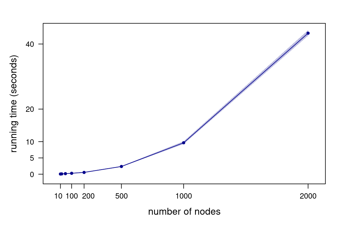

Figure 4.4: Running times for Algorithm 4.1 as a function of the number of nodes, generating 200 DAGs.

How do time and space complexity change if we represent DAGs with adjacency lists instead? Both path finding (say, by depth-first search) and saving DAGs in a different data structure have a time complexity of \(O(|\mathbf{V}| + |A_n|)\) for adjacency lists. However, the overall time complexity of each MCMC iteration is still quadratic: \[\begin{multline*} O\left(N \left(1 + 1 + (|\mathbf{V}| + |A_n|) \frac{|A_n|}{|\mathbf{V}|^2}\right)\right) \approx \\ O\left(N \left(1 + 1 + (|\mathbf{V}| + |\mathbf{V}|^2) \frac{|\mathbf{V}|^2}{|\mathbf{V}|^2}\right)\right) \approx O(N|\mathbf{V}|^2), \end{multline*}\] again assuming that \(O(|A_n|) \approx O(|\mathbf{V}|^2/4)\). The space complexity of an adjacency list is \(O(|\mathbf{V}| + |A_n|)\). On average, this becomes \(O(|\mathbf{V}|^2)\) under the same assumption.

4.6 Big-\(O\) Notation and Real-World Performance

Big-\(O\) notation is a useful measure to assess scalability, and it can often be related to the practical performance of real machine learning software. However, this becomes increasingly difficult as such software becomes more complex, for several reasons. For instance:

• Software in a machine learning pipeline is heterogeneous: various parts are typically written in different programming languages and are built on different libraries. Each part may be faster or slower than another because of that, even when they belong to the same class of complexity. More on that in Section 6.1. Software upgrades may also change the relative speeds of different parts of the pipeline and introduce new bottlenecks.
• Both these things being equal, the same algorithm may be faster or slower depending on the data structures used to store its inputs and outputs. We saw that to be the case in Section 4.5.2, and we touched on this point in Section 3.4 as well. The same is true for variable types, as discussed in Section 3.3. High-level languages abstract these details to a large extent, which may lead to surprises when benchmarking software.
• Differences in hardware can be impactful enough to completely hide differences in the class of complexity of different algorithms for practical ranges of input sizes. Conversely, they can also introduce apparent discrepancies in performance. This can realistically happen when the input sizes are small enough to make adjacent classes of complexity comparable: an \(O(N^2)\) algorithm on a CPU core will be slower than an \(O(N^3)\) algorithm on a GPU with a hundred of free units for \(N \leqslant 100\). Fixed costs that are ignored when deriving computational complexity may also be relevant due to the relative difference, for instance, in the latency of different types of memory (Section 2.1.2).
• If we use any remote systems (Section 2.3), the hardware we are running a machine learning pipeline on may vary without our knowledge, either in its configuration or in its overall load. Furthermore, benchmarking remote systems accurately is inherently more difficult, as is troubleshooting them.
• The performance of some parts of the pipeline may be artificially limited by that of the external systems that provide the inputs to the machine learning models or that consume their outputs. Individual parts of the same system may also slow down each other as they consume each other’s outputs.

To summarise, we may be able to map computational complexity to real-world performance for the individual components of a machine learning pipeline running on simple hardware configurations. It is unlikely that we can do that with any degree of accuracy when systems become larger and contain a larger number of software and hardware components. The resulting complexity can easily make our expectations and intuitions about performance unreliable. In such a situation, identifying performance issues requires measuring the current performance of each component as a baseline, identifying which components are executed most often (which are sometimes said to be in the “critical path” or in the “hot path”) and trying to redesign them to make them more efficient.

References

Bates, D., and M. Maechler. 2021. Matrix: Sparse and Dense Matrix Classes and Methods. https://cran.r-project.org/web/packages/Matrix/.
Gelman, A., B. Carlin, H. S. Stern, D. B. Dunson, and A. Vehtari. 2013. Bayesian Data Analysis. 3rd ed. CRC Press.
Goodfellow, I., Y. Bengio, and A. Courville. 2016. Deep Learning. MIT Press.
Knuth, D. E. 1976. “Big Omicron and Big Omega and Big Theta.” ACM Sigact News 8 (2): 18–24.
Knuth, D. 1997. The Art of Computer Programming, Volume 1: Fundamental Algorithms. 3rd ed. Addison-Wesley.
McConnell, S. 2004. Code Complete. 2nd ed. Microsoft Press.
Melançon, G., I. Dutour, and M. Bousquet-Mélou. 2001. “Random Generation of Directed Acyclic Graphs.” Electronic Notes in Discrete Mathematics 10: 202–7.
Montgomery, D. C. 20AD. Design and Analysis of Experiments. 10th ed. Wiley.
Santner, T. J., B. J. Williams, and E. I. Notz. 2018. The Design and Analysis of Computer Experiments. 2nd ed. Springer.
Scikit-learn Developers. 2022. Scikit-learn: Machine Learning in Python. https://scikit-learn.org/.
Scutari, M., and J.-B. Denis. 2021. Bayesian Networks with Examples in R. 2nd ed. Chapman & Hall.
Tsay, R. S. 2010. Analysis of Financial Time Series. 3rd ed. Wiley.
Virtanen, P., R. Gommers, T. E. Oliphant, M. Haberland, T. Reddy, D. Cournapeau, E. Burovski, et al. 2020. “SciPy 1.0: Fundamental Algorithms for Scientific Computing in Python.” Nature Methods 17: 261–72.
Weisberg, S. 2014. Applied Linear Regression. 4th ed. Wiley.
Wikipedia. 2021a. Cholesky Decomposition. https://en.wikipedia.org/wiki/Cholesky_decomposition.
Wikipedia. 2021b. Matrix Multiplication Algorithm. https://en.wikipedia.org/wiki/Matrix_multiplication_algorithm.
Wikipedia. 2021c. QR Decomposition. https://en.wikipedia.org/wiki/QR_decomposition.
This assumes that each row of \(\mathbf{X}\) corresponds to a data point and that each column corresponds to a variable. Sometimes these dimensions are inverted (variables on the rows, data points on the columns) in the literature.↩︎
We can do better, but not much: combining Gram-Schmidt and Householder transformations gives \(O(rs^2 - s^3/3)\).↩︎